Charts

In this page

How to create Excel charts from Jira data?

Defining the source data

We will explain charts through a very simple example: displaying the time spent per issue in a horizontal bar chart.

First you need to produce the source data that you wanted to visualize in the Excel spreadsheet. You can use formulas, functions, tags, scrips and all other tools to render the source data.

Instructions for Excel:

1. Create a new spreadsheet.
2. Rename the first sheet to "Issues".
3. Export the issue key in the first column and the timeSpent property in the second.
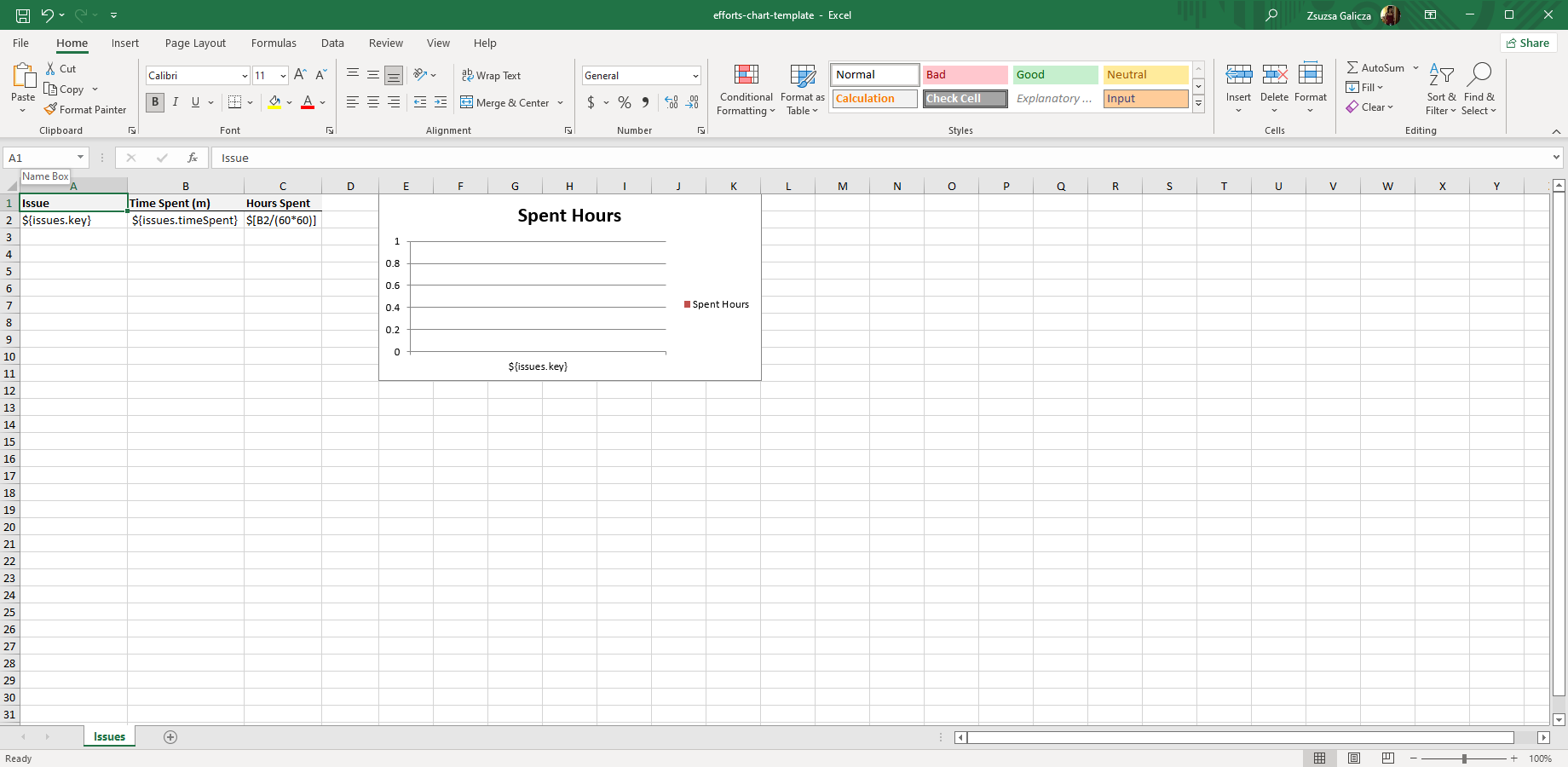
   Thus, the sheet for the source data would be as simple as:

   | Issue         | Time Spent (sec)    | Hours Spent (h) |
   | ${issues.key} | ${issues.timeSpent} | $[B2 / (60*60)] |

Defining the data ranges

When you have the source data template defined, you also need to define so-called named dynamic ranges. A named dynamic range is a rectangular block of cells, that dynamically expands to cover the source data. Ranges are identified by their names. We will define two separate ranges, one for each column, and use those later as the input for our chart.

Instructions for Excel:

1. Go to Formulas → Name Manager.
2. Click New and enter the name "Keys".
3. Enter the following expression to the "Refers to" inputbox:

   =OFFSET($A$2,0,0,COUNTA($A$2:$A$9999),1)

   It requires some explanation.
   The OFFSET() function defines a so-called cell range, a rectangular block of cells, specified by its top-left corner, its height and width. Its arguments:
   1. The reference cell. Make the "A2" cell the reference cell, because "A1" contains the header text "Issue", which we want to exclude.
   2. Vertical offset, relative to the reference cell. Use zero to make "A2" the top-left cell of the range.
   3. Horizontal offset. See previous.
   4. Number of rows for the range. To specify this value, we use another function called COUNTA(). This function will calculate how many cells in the column "A" (cell range from A2 to A9999) has no-empty value.
   5. Number of columns.
4. Now you created a range that will span over the first column (excluding the first row).
5. Create another range for the 3rd column (spent hours), but use the name "Hours" and the formula:

   =OFFSET($C$2,0,0,COUNTA(Issues!$C$2:$C$9999),1)

It may sound difficult first, but it is actually totally trivial.

Hint: later you will be able to easily test whether your ranges are correctly defined. After you make an export, open the resulted spreadsheet, go to Name Manager, click one of the ranges and click the "Refers to" box. The rectangle of the range will be highlighted!

Defining the chart

With the ranges in place, you can finally create your chart by selecting that as input data. Note that as there is no real data in your template, the chart in the template will not contain any meaningful graphics. Although it is blank, you can configure it, specifying its type, look, title and so on.

Instructions for Excel:

1. Go to Insert.
2. Insert a column chart (any type will do).
3. Click Select Data in the Design ribbon.
4. Click Add in the "Legend Entries (Series)" box. Enter "Spent Hours" as "Series name" and "=Issues!Hours" as "Series values".
   Please note that "Issues" is the name of your worksheet and "Hours" is the name of the dynamic range that specifies the size of the bars in the chart.
   (If there is another entry in this box, delete that.)
5. Similarly, click Edit in the "Horizontal (Category) Axis Labels" and enter "=Issues!Keys" as "Axis label range".
   This will specify the display label for bars.

Now your part is done.

Exporting the chart

You can make an export now:

1. Upload your template to the app.
2. Create a new view named "Times Spent Report (Excel)" for this new template. Enable it for at least the "Issue Navigator" context (or set the "Multiple Issues" type in pre-2.2.0 versions).
3. Run a JQL query that returns a list of issues.
4. Export the result using your new view.

Yay, what a wonderful chart!

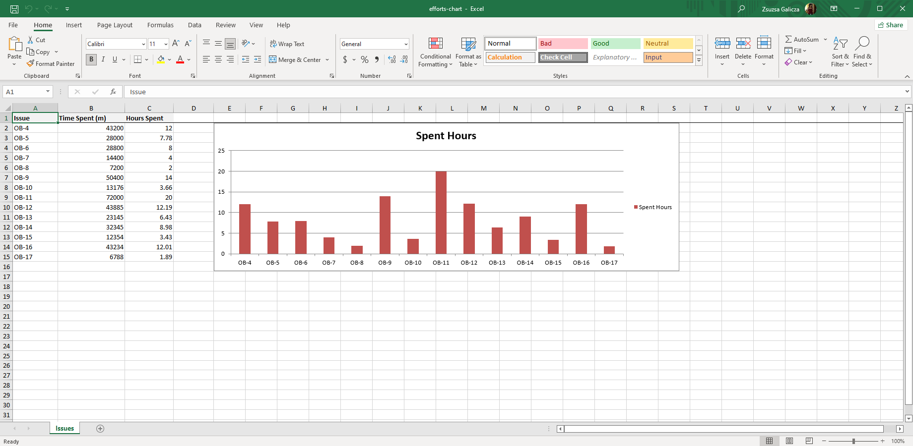
What happens in the background? During the export, the app will fill the source data cells with actual data. Then, as soon as you open the spreadsheet in Excel, it will find the named data range and display your chart.

Enjoy your chart!

Video tutorial

There is a section in the app's introductory video, that goes through creating a custom report with a bar chart. This demonstrates the steps above in action. Grab a cup of coffee, enable the subtitles and enjoy!

Resources

efforts-chart-template.xlsx — a sample Excel template to generate charts. Use this for your experiments.

Next step

Create Excel pivot tables for interactive analysis of your Jira data.

Questions?

Ask us any time.