Pivot Tables

In this page

What is a pivot table?

Pivot tables are really powerful tools for data analysis. They can quickly summarize large sets of data, sort and count that, calculate sum, average, minimum, maximum and other aggregate values. They also allow users to "drill down" the data to desired scope (e.g set the time resolution from year level to month level) and to filter data entries (e.g. only calculate for "bug" type issues).

In Excel, all these operations are really easy, mostly available via drag and drop.

Excel pivot table tutorials

There are many great tutorials about Excel pivot tables in the web. Here is a collection of resources that we found useful:

• "Pivot table" article in Wikipedia — to get a general overview.
• Create or delete a PivotTable or PivotChart report — the official tutorial in the Excel documentation (by Microsoft).
• Google for "Excel pivot table" — to find videos and tutorials for various experience levels.

How to create Excel pivot tables from Jira data?

Defining the source data

First you need to render the source data in the Excel spreadsheet. We suggest you create a separate worksheet for the source data, with a one-line fixed header and add one row for each data record. You can use formulas, functions, tags, scrips and all other tools to render the source data.

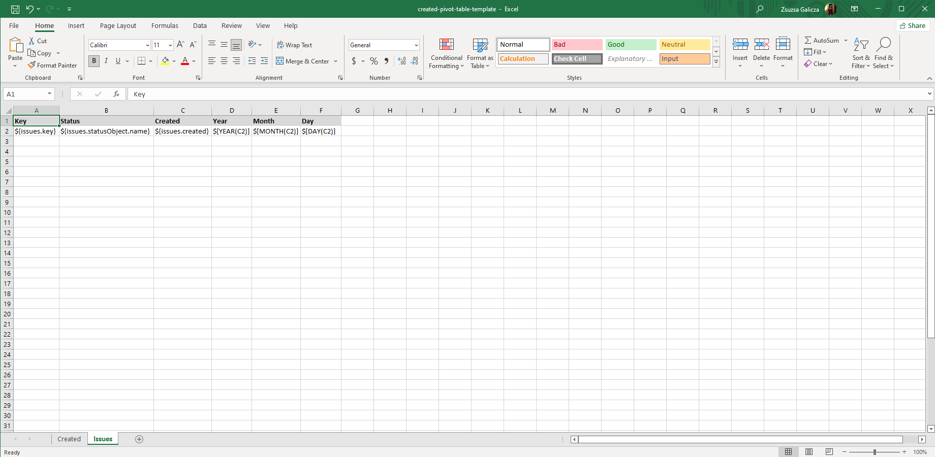
In this example, we will guide you through a simple pivot table example of analyzing current issue status counts by creation date.

Instructions for Excel:

1. Create a spreadsheet.
2. Rename the last sheet to "Issues".
3. Export the issue key in the first column, export the issue status' name in the second, the creation date in the third (set the type of this sell to "Date"), and extract the creation year / month / day components using Excel formulas in the last three columns:

   | Key           | Status                      | Created                                       | Year        | Month        | Day        |
   | ${issues.key} | ${issues.statusObject.name} | ${issues.created} | $[YEAR(C2)] | $[MONTH(C2)] | $[DAY(C2)] | 

Defining the data range

When you have the source data template defined, you also need to define a so-called named dynamic range. A named dynamic range is a rectangular block of cells, that dynamically expands to cover the source data. Ranges are identified by their names. We will define a single range, and use that later as the input for our pivot table.

Instructions for Excel:

1. Go to Formulas → Name Manager.
2. Click New and enter the name "Creations".
3. Enter the following expression to the "Refers to" inputbox:

   =OFFSET($A$1,0,0,COUNTA($A$1:$A$9999),6)

   It requires some explanation.
   The OFFSET() function defines a so-called cell range, a rectangular block of cells, specified by its top-left corner, its height and width. Its arguments:
   1. The reference cell. Make the "A1" cell the reference cell.
   2. Vertical offset, relative to the reference cell. Use zero to make "A1" the top-left cell of the range.
   3. Horizontal offset. See previous.
   4. Number of rows for the range. To specify this value, we use another function called COUNTA(). This function will calculate how many cells in the column "A" (cell range from A1 to A9999) has no-empty value.
   5. Number of columns. We exported 6 columns and want to include all of them in the range.

Hint: later you will be able to easily test whether your ranges are correctly defined. After you make an export, open the resulted spreadsheet, go to Name Manager, click one of the ranges and click the "Refers to" box. The rectangle of the range will be highlighted!

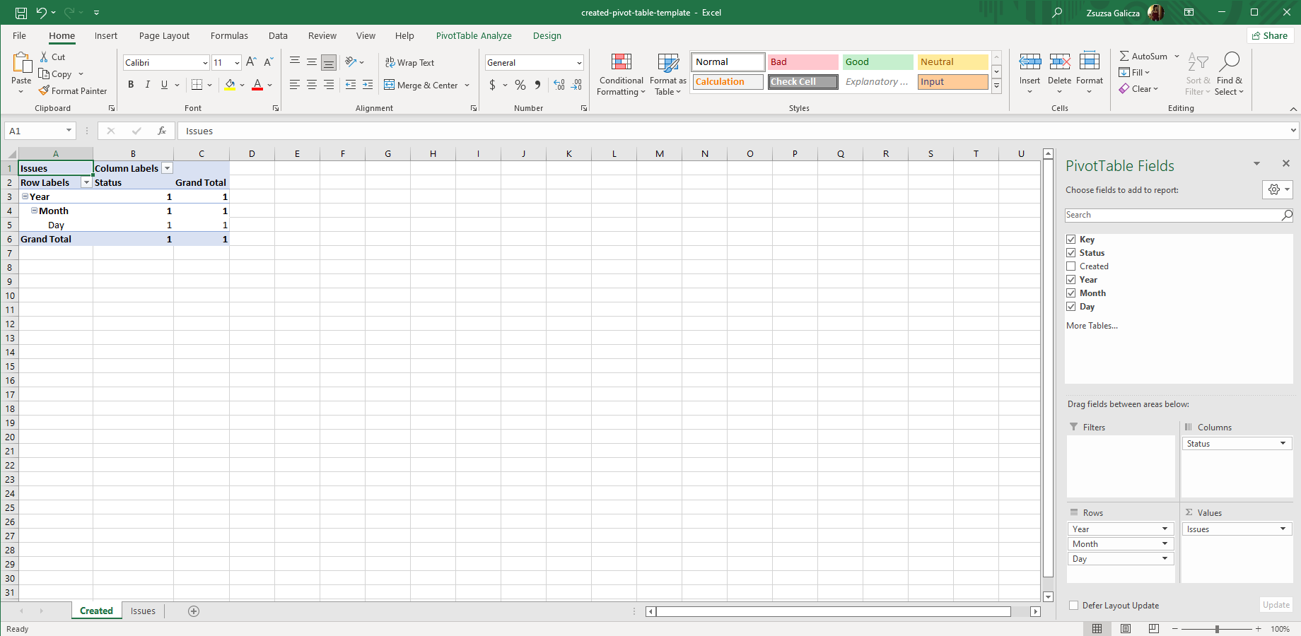
Defining the pivot table

With the ranges in place, you can finally create your pivot table by selecting those as input data. Note that as there is no real data in your template, the pivot table in the template will not contain any meaningful figures. Although it is blank, you can configure it, specifying its columns, rows, filters, look, and so on.

Instructions for Excel:

1. Go to Insert → PivotTable.
2. Enter "Issues!Creations" to the Table/Range input box.
   Select the New Worksheet option to place the pivot table in its own worksheet.
3. Now your empty pivot table appears. By drag and dropping the field names between the boxes in the Pivot Table Field List bar, set up these:
   1. Add "Status" to Column Labels.
   2. Add "Year", "Month" and "Day" (in this order) to Row Labels.
   3. Add "Count of Key" to ∑ Values.
4. At this point, you need to rewrite the generated pivot cell content a little. Not only it will make them more readable, it will also prevent rendering errors caused by the automatically generated placeholders.
   Replace the following placeholder texts:
   1. Replace the pivot cell text "$[YEAR(C2)]" with "Year", and similarly for "Month" and "Day".
   2. Replace the pivot cell text "${issues.statusObject.name}" with "Status".
5. In order to set the correct sorting for the date components, right-click each of the "Year", "Month", "Day" cells and click Sort → More Sort Options and select the Ascending option.
6. Go to the Pivot Table ribbon → Pivot Table Options → Data tab:
   1. Check the Refresh data when opening the file checkbox. This way Excel will auto-refresh your pivot table after the template is merged with actual data.
   2. Still in the Data tab, set the Number of items to retain per field setting to None. This will ensure that no mysterious, deleted expressions appear in the pivot table's filter drop-downs.

Now your part is done.

Exporting the pivot table

You can make an export now:

1. Upload your template to the app.
2. Create a new view named "Status by Creation Date (Excel)" for this new template. Enable it for at least the "Issue Navigator" context (or "Multiple Issues" in pre-2.2.0 versions).
3. Run a JQL query that returns a list of issues.
4. Export the result using your new view.

Yay, what a wonderful pivot table!

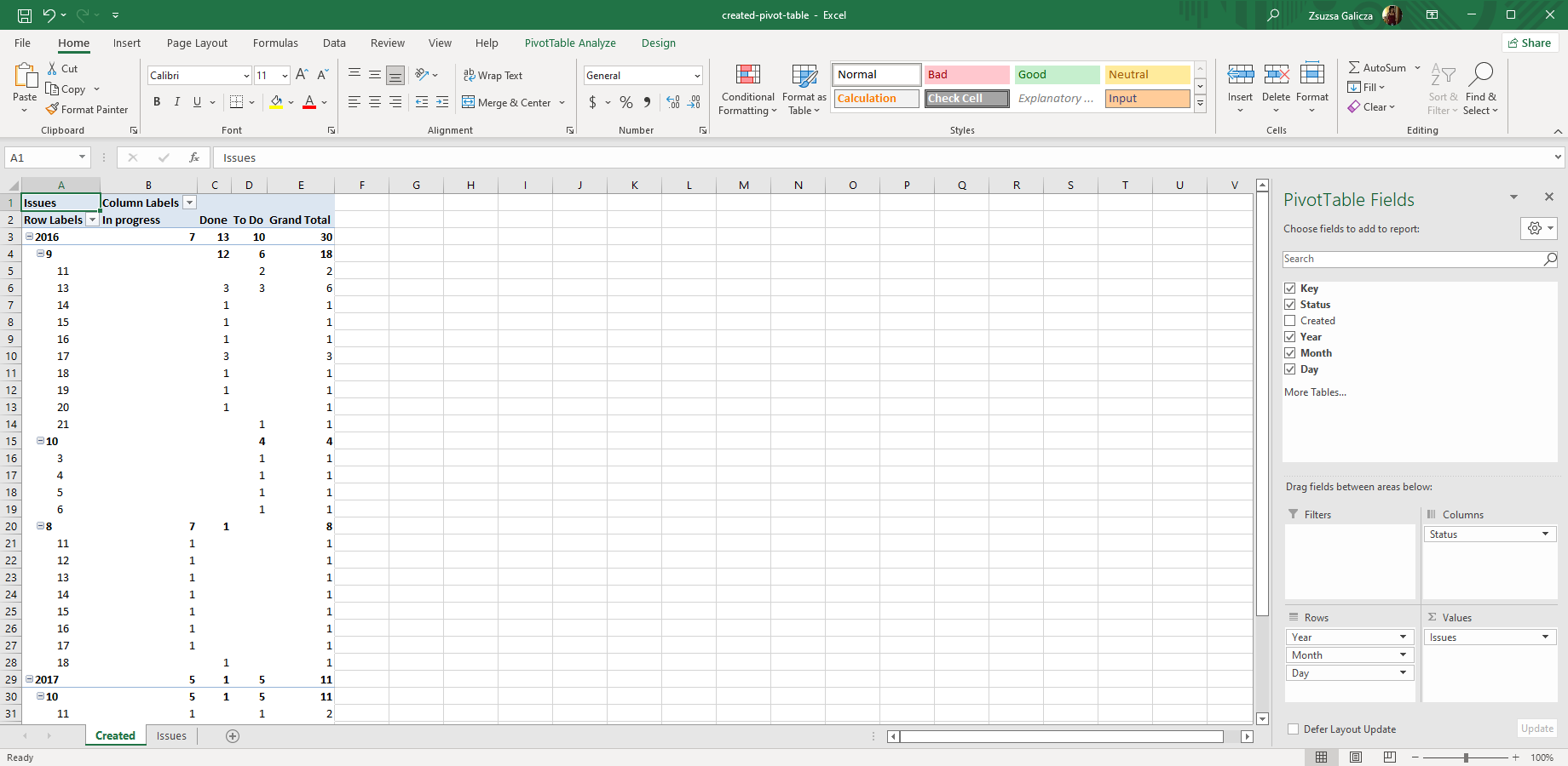
What happens in the background? During the export, the app will fill the source data cells with actual data. Then, as soon as you open the spreadsheet in Excel, it will find the named data range and display your pivot table.

Working with the pivot table

Pivot tables are really powerful. Experiment with the tons of interactive features in Excel, for instance:

• Click the pivot cells (the ones with the numbers) and Excel will create you a new worksheet listing the issues corresponding to that filtering criteria.
  For example, if you the click the intersection of the "Open" column and the "2014 Jan" row, Excel will list you the open issues created in that month. Whoa, one click reports!
• Expand and collapse the "Month" and "Day" rows, or completely drop the "Day" field to change the report's resolution.
• Click the "Status" field in the Pivot Table Field List bar and uncheck everything, but the "Open" and "In progress" items. This will filter your data to show only the outstanding work!
• Export further data like assignee name, project name, issue type and implement new pivot tables that match your needs.

Enjoy your pivot table!

Resources

created-pivot-table-template.xlsx — a sample Excel template to generate pivot tables. Use this for your experiments.

Next step

Display Excel pivot charts to comply your pivot tables, because as data scientists say "a chart is worth a million numbers" (OK, not exactly like that).

Questions?

Ask us any time.